


The Effect of Dimensioning Computer Models

Coding a computer model to simulate something in the real world requires compromises. The compromises scientists must make have to balance accuracy, detail and computer resources. This becomes increasingly difficult as the problem being modeled becomes more and more complex. After decades of modeling, scientists and programmers have become very good at making these compromises, but not as effective at communicating the uncertainty introduced in the process. I’d like to give the reader a brief description of how these compromises are made and what effect they can have on predictions of climate change and other important topics.
One area of compromise comes up when dimensioning the model. A computer model simulating star formation or stellar evolution will choose enormous time steps, on the order of millions of years. But if a scientist is interested in chemical reactions in the ocean, the simulation should have smaller time increments, perhaps as short as seconds. The trick is to pick a time increment that will provide the appropriate detail for the situation without wasting computer resources.
Spatial dimensioning is equally tricky. Models that deal with geographic areas typically rely on grids of equal area. It is often necessary to change the grid dimensions, however, in areas where more detail is required. Someone modeling traffic congestion might be able to get away with 100 m grids on the interstate between major cities but would need to transition to smaller grids near suburbs (25 m) and major cities (5 m).
Modeling the atmosphere benefits by changing from equal length to equal pressure. The models operate more efficiently if the atmosphere is divided this way. It provides fine detail where the pressure is highest near the ground but calculates thicker layers as pressure drops in the upper atmosphere.
One Compromise in RF Engineering Models
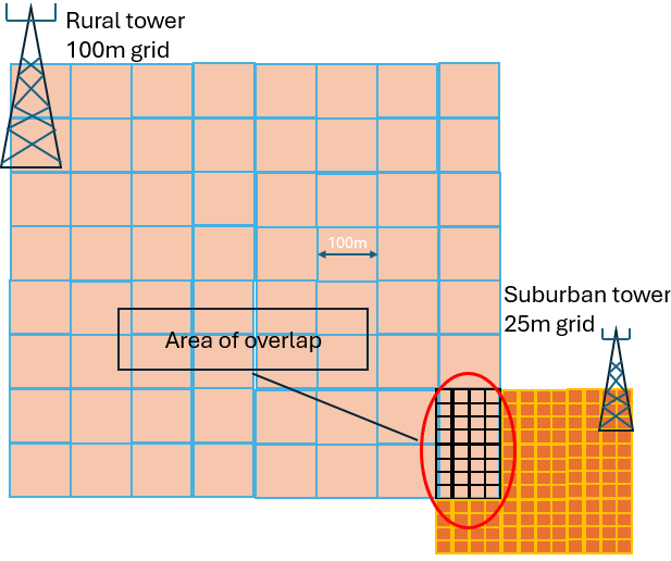
I am familiar with this type of compromise and its effect on simulation results because of the work I do as an RF engineer. In my job, I must predict the radio signal strength coming from a tower over a wide geographic area. The models that calculate these predictions rely on dividing the terrain into square grids and then predicting the signal strength for the point in the center of the grid. The grid size used to make predictions varies based on the area being modeled. The model will use a coarse 100m grid for predictions covering rural areas, 25m grid for suburban neighborhoods and 5m grid for urban settings. The 5m urban grids provide the details necessary to evaluate coverage. It is important to see if the left side of an intersection has the same signal level as the right side in an urban setting. As the model moves out to the rural areas, that level of detail is wasted effort. Since there isn’t much of interest along a highway or in a farmer’s field, predictions only have to be made for areas the size of a football stadium.
This compromise is done for the sake of efficiency but creates inaccuracies where predictions overlap. In the illustration below, there is a tower with a 100m grid that overlaps with a suburban prediction using a 25m grid. There 16 predicted signal levels for the suburban tower in each 100m rural prediction. To determine which signal is strongest, the model repeats the rural tower signal strength in each 25m suburban grid and compares the two. The strongest signal serves the geographic area inside that 25m grid. This isn’t entirely accurate, however, since the signal from the rural tower will vary within that 100m geographic area. The compromise has led to this inaccuracy. A good engineer realizes this and treats the results in overlapping areas with some caution.
Today’s cellular technologies are interference limited, meaning that it is more important that the serving tower have a signal that is stronger than any other signal in the background. It’s analogous to waking up in a quiet room and hearing your partner whisper to you. You would never hear that same whisper while out shopping. The background noise (interference) would be too loud.
RF engineers refer to this as signal to noise ratio (SINR) and it is a key metric used to determine if an area will provide good service or not. SINR is a comparison of the signal strength serving the device versus all the other signals in the same frequency range (interference). If the rural site is serving the user in a bin, then signal from the suburban tower is treated as interference (and vice versa if the suburban site is serving).
These areas of overlap in the model decrease the accuracy of the SINR predictions by as much as 15% to 30%. The model can be adjusted to predict the rural sites at 25m resolution but that would mean waiting 16 times longer for the results. Day-to-day engineering tasks don’t have that kind of time. So, good engineers understand that it is better to be conservative when evaluating areas of overlap.
One Compromise in Climate Models
Climate models run into a similar problem when modeling clouds. The formation of clouds occurs on a scale that is smaller than the grids used in climate models. It is understandable when one considers the amount of data being calculated in these models.
Climate models need to predict temperature, rainfall, cloud cover and dozens of other factors. The models must cover the entire globe, so the grid space must be on the order of kilometers. Then consider these models are predicting in 3 dimensions because the climate includes layers of the atmosphere above and layers of the ocean below. Judith Curry gives us an idea of the scope in a 2017 briefing.
“Common resolutions for GCMs [General Circulation Models] are about 100–200 km in the horizontal direction, 1 km vertically, and a time-stepping resolution typically of 30 min.”
In rough numbers, the earth has a surface area of 510 million square kilometers. If I lay out a grid across that surface, 100 km on a side, I will need 5.1 million squares to cover the surface of the globe. The atmosphere above the surface will have 20, one kilometer grids with roughly the same number of squares as the surface. That brings us to 102 million squares to calculate.
Within each of these, the model has to determine the chemical composition of the air, how much heat is absorbed by the land, how much heat is released to the atmosphere and how much is absorbed by each layer, how much water is evaporated and subsequent cloud formation, air circulation vertically and horizontally, humidity, and on and on. Many of these calculations aren’t simple math, either. They can each take a significant amount of time.
Let us just say there are 2 dozen factors that are calculated for each grid. That brings us to 2.5 billion calculations. But that represents just a single time step of 30 minutes. One year carved up in 30 minute segments means the model has to perform 17,500 iterations to complete one year. We are now looking at roughly 43 trillion calculations to complete one year of climate model predictions.
Obviously, compromises must be made to produce a model that will make these predictions in a reasonable amount of time. Let me explain how these compromises affect the treatment of clouds.
Clouds are incredibly important in climate because different types of clouds have different effects. Cirrus clouds, those high wispy clouds seen on sunny days, allow sunlight through to heat the planet. But the ice crystals that make them up tend to trap heat. So, Cirrus clouds act as positive warming feedback to the models. Cumulus clouds, low puffy clouds, block the sun and reflect light back to space. These clouds generally cool the planet. So, you would think that modeling the number and types of clouds covering the planet would be a key factor in climate models. Unfortunately, the compromises in grid size prevent the models from accurately representing clouds.
Below, I have sketched a single block from a model and drawn the two cloud types. It is clear that the prediction block is much larger than the clouds. This is why they cannot be accurately modeled. For scale, I’ve laid out a 100km grid over a US metropolitan area. Anyone who has watched a weather radar understands that cloud cover will be patchy over a large area like this. There could even be different types of clouds at each end of the grid.

Scientists have compromised by parameterizing clouds in the model. This involves estimating cloud cover based on other calculated parameters like humidity and other factors. From this information, the model will treat a grid as clear sky if the humidity is below a certain value. If humidity reach a value between X and Y, it will treat the grid as having say 30% cirrus cloud cover and over humidity Y 50% cumulus cloud cover (just as an example).
This is not a flaw in the models. It is a compromise that introduces errors into the final predictions. In a future essay, I intend to dive deeper into how much this error may or may not affect the final predictions. For now, it is understood that the cloud parameterization may misrepresent the actual cloud cover by as much as 30%. This should not be controversial since it was admitted in one of the IPCC reports.
Using Predictions to Make Decisions
The engineering model I use for my job helps me make $500,000 decisions. It is important that I keep this in mind as I review the predictions. I need to be certain that the tower will cover the land area targeted by the project. Perhaps a suburban shopping mall is targeted for coverage and I misinterpret predictions. The errors inherent in the model dimensioning could mean the predictions show the mall is covered if the tower is built at a location. But when the tower is turned up, we find it doesn’t have sufficient signal strength to get inside the building. If that happens, $500k was just wasted.
More often, the project is initiated to add capacity to an area. In these instances, the area under the new tower has adequate coverage from existing near-by towers. The problem is that customers are complaining of slow connection speeds. The new tower will add greater bandwidth and hence improve the speed.
But this comes at a cost. Recall that today’s 4G and 5G technologies are interference limited. Reviewing the model predictions, I must pay special attention to SINR in these cases because the new tower could degrade the service by adding interference to areas that don’t have interference today. If I don’t account for the 15% to 30% error in SINR predictions, I may approve the location only to find out in reality that tower causes all kinds of interference in a key area. Again, $500k was spent to solve a problem, but it created a new problem over here.
I highlighted just one error introduced to climate models by the dimensioning of models. I focused on how the clouds are treated in the models because they have a substantial influence on the end results. The IPCC puts the cloud error at ~30%, yet politicians are making decisions that could cost us all billions of dollars. And there is still considerable debate in the scientific community about how to model them and tune the parameters. You would never know this given the confident presentation in the media.
I go through this description to show that computer models are helpful in making decisions in the real world. But they can’t be taken as actual representations of the real world. This is something the media, pundits and unfortunately some scientists don’t communicate very well. Please keep this in mind as you consume science news, especially if it is covering controversial topics like climate science or epidemics.